Introduction
In this blog post we’re going to take a deep dive into support vector classification (SVC) in Python. We will start by looking at the basics of SVC and how it works, before moving on to discuss some of its most important features and parameters. Finally, I’ll show you how easy it is to implement SVC with sklearn for your own machine learning projects. Let’s get started!
Table of Contents:
- Support Vector Machine Classification Use Cases
- How Support Vector Machine Classification Works
- How Support Vector Machines work for Binary Classification in Python
- Pros and Cons of Support Vector Machines for Classification
- Conclusion

Your FREE Guide to Become a Data Scientist
Discover the path to becoming a data scientist with our comprehensive FREE guide! Unlock your potential in this in-demand field and access valuable resources to kickstart your journey.
Don’t wait, download now and transform your career!
Support Vector Machine Classification Use Cases
There are many use cases for using SVC, for example:
- Detecting Fraudulent Transactions: SVM can be used for identifying whether a financial transaction is legitimate or not.
- Text categorization (spam detection): SVMs may be used to differentiate between emails that are normal vs those categorized as spam using various features such as the presence of particular words, phrases, symbols and numbers etc., within the body of an email message or its header information and using them as input parameters for training data set to create output values which can then classify mail according to specific categories.
- Bioinformatics: In bio-medical fields like Genomics and Proteomics, Support Vector Machine Algorithms have been applied for applications such as gene expression analysis , cancer classification, DNA sequencing etc.. By combining multiple biological data types at once the algorithm is effectively able to find relationships between diseases states & gene expression levels – something much more difficult when observed singly due their complexity.
- Malware Detection and Categorization: SVM can differentiate between malicious software and ‘clean’ software using its pattern recognition abilities to classify the two types accurately.
Let’s get an understanding of how the basics of SVCs work.
How Support Vector Machine Classification Works
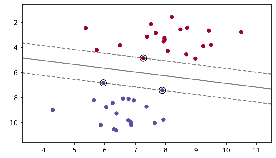
Support Vector Machines (SVMs) are supervised machine learning algorithms used for classification problems. SVMs work by mapping data to a high-dimensional feature space so that data points can be categorized based on regression or classification in two dimensions. The algorithm creates an optimal hyperplane that divides the dataset into two classes, and then uses support vectors as its building block for classifying new data observations. Support vectors are the data points nearest to the hyperplane, meaning their influence is greater compared to other observations further away from the model boundary.
During the training phase of an SVM model, it tries to make sure that all distance between any two distinct categories is maximized while making sure no point lies on any wrong side of decision boundary which leads to misclassification penalty. While doing this at different angles and sizes, it finds a line segment that works as best boundary – which is called Maximal Margin Classifier (MMC). This optimal hyperplane will also avoid overfitting thereby improving generalization performance when predicting future unseen data instances slightly differently than already seen outliers in sample set.
Here we can see a visualization of a separating hyperplane and the support vectors, with a dashed line to show the margin:
How Support Vector Machines work for Binary Classification in Python
Let’s explore a simple example of using Support Vector Machines with Scikit-Learn and Python on a binary classification problem, which is when we have only 2 classes to distinguish or predict given a set of features. We’ll use a Social Network Advertising dataset from Kaggle, which can be found and downloaded here: https://www.kaggle.com/datasets/rakeshrau/social-network-ads?resource=download
Let’s begin with some imports and grabbing a subset of features (this will allow us to actually visualize the hyperplane separation in some plots.
# Importing the libraries
import numpy as np
import matplotlib.pyplot as plt
import pandas as pd

# Importing the dataset
dataset = pd.read_csv('Social_Network_Ads.csv')
X = dataset.iloc[:, [2, 3]].values
y = dataset.iloc[:, 4].values

# Splitting the dataset into the Training set and Test set
from sklearn.model_selection import train_test_split
X_train, X_test, y_train, y_test = train_test_split(X, y, test_size = 0.25, random_state = 0)

# Feature Scaling
from sklearn.preprocessing import StandardScaler
sc = StandardScaler()
X_train = sc.fit_transform(X_train)
X_test = sc.transform(X_test)

# Fitting SVM to the Training set
from sklearn.svm import SVC
classifier = SVC(kernel = 'linear', random_state = 0)
classifier.fit(X_train, y_train)

# Predicting the Test set results
y_pred = classifier.predict(X_test)

# Making the Confusion Matrix
from sklearn.metrics import confusion_matrix
cm = confusion_matrix(y_test, y_pred)
Now let’s take a look at the results by plotting out our Confusion Matrix:
from sklearn.metrics import confusion_matrix, ConfusionMatrixDisplay
disp = ConfusionMatrixDisplay(confusion_matrix=cm,display_labels=classifier.classes_)
disp.plot()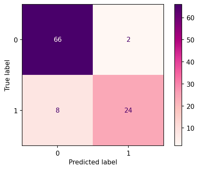
We can also develop visualizations for the hyperplane, since we used a linear kernel:
# Visualising the Test set results
from matplotlib.colors import ListedColormap
X_set, y_set = X_test, y_test
X1, X2 = np.meshgrid(np.arange(start = X_set[:, 0].min() - 1, stop = X_set[:, 0].max() + 1, step = 0.01),
                     np.arange(start = X_set[:, 1].min() - 1, stop = X_set[:, 1].max() + 1, step = 0.01))
plt.figure(dpi=150)
plt.contourf(X1, X2, classifier.predict(np.array([X1.ravel(), X2.ravel()]).T).reshape(X1.shape),
             alpha = 0.75, cmap = ListedColormap(('#8142f5', '#f5425c')))
plt.xlim(X1.min(), X1.max())
plt.ylim(X2.min(), X2.max())
for i, j in enumerate(np.unique(y_set)):
    plt.scatter(X_set[y_set == j, 0], X_set[y_set == j, 1],
                c = ListedColormap(('#8142f5', '#f5425c'))(i), label = j)

plt.title('SVM (Test set)')
plt.xlabel('Age')
plt.ylabel('Estimated Salary')
plt.legend()
plt.show()
This will result in the visualization of the linear hyperplane on the test set, notice how there are some misclassifications (which is to be expected on a real world data set):
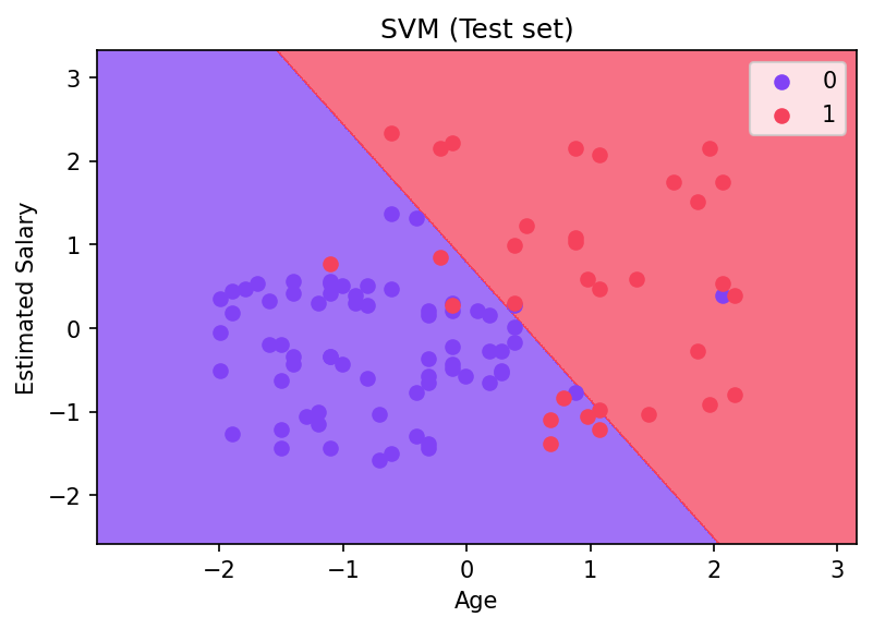
Very cool! We can see the hyperplane separating classes based off the salary and age features, two of the strongest features in the dataset, you may want to try to repeat this exercise and use more features (keep in mind you can really visualize a high dimensional hyperplane!)
Pros and Cons of Support Vector Machines for Classification
Let’s discuss the advantages and disadvantages of using SVMs for classification.
Pros
- Highly Efficient and Robust: Support vector machines utilize high-dimensional feature spaces which make them robust to minor errors or slight variations in the data that could affect other methods such as decision trees. Furthermore, they are resistant to overfitting of training data without excessively reducing accuracy.
- Effective in High Dimensions: Unlike naïve Bayes or logistic regression approaches, SVM scales well with larger datasets by cleverly searching only select examples within a given dataset for constructing its hyperplanes rather than every example like other techniques do; i.e., it possesses much greater computational efficiency when working with higher dimensional input data compared against any nonlinear classifiers for classification tasks with more than two classes (also referred to as multinomial problems).
- Not Restricted to Linear Class Separations: One of the biggest advantages is that support vector machines can handle nonlinear boundary cases through their kernel trick transformations that allow even complex boundaries and functions which would otherwise be impossible for linear models like linear/logistic regression or traditional neural networks as discussed earlier preceding this point in detail.
- Wide Range Of Kernel Options: With many algorithms emerging for better machine learning performance – Support Vector Machines provides wide range of external tools including varying kernel options & user-defined kernels such as radial basis function(RBF), etc., helping create customized solutions aiding research projects more efficiently!
- Flexible hyperparameter tuning: This enables one to explore various combinations of hyperparameters for Support Vector Machines, allowing for more efficient optimization of a model’s performance. It can help identify and select the most appropriate values for all or some of the parameters found in an SVM algorithm. This helps increase predictive accuracy and optimize models better.
Cons
- Memory Usage: It requires a lot of memory and computational resources: Support Vector Machines are resource-intensive algorithms which require a large amount of RAM as well as substantial CPU time. This makes them less suitable for larger datasets or real-time applications.
- Limited Kernel Functions: Support Vector Machines currently have limited kernel functions available for classification tasks, therefore making it difficult to use in certain cases where more complex kernels can be used to help classify data better than simpler ones will allow for.
- High Variance: Due to their complexity, they also tend to overfit the training data which results in high variance and poor generalization ability on unseen samples from the same distribution as the training set was drawn from. This means that hyperparameter optimization must be done carefully when using SVM classifiers in order to achieve optimal performance within the desired domain.
- Semi-Blackbox Nature: SVMs provide fewer interpretability options compared with other machine learning models like decision trees, logistic regression etc., thereby making it difficult to explain their decisions or predictions – especially when involving more complex nonlinear parameters -which further prevents informed decision-making by stakeholders relying on its outputs
Conclusion
Overall, support vector machine classification is a powerful tool that can bring great accuracy to your project. With the right data and some experience with the Python programming language, you will be able to use this technique easily and efficiently to create superior models and get better results. With its scalability and robustness in dealing with complex datasets, it’s no wonder why SVM continues to stay popular among data scientists. If you’re looking for an effective way of classifying large amounts of information, look no further – SVM is here for you!
Interested in learning more about Machine Learning in Python, check out our courses and training sessions!