Regression analysis is a commonly used statistical technique for predicting the relationship between a dependent variable and one or more independent variables. In the field of machine learning, regression algorithms are used to make predictions about continuous variables, such as housing prices, student scores, or medical outcomes. Python, being one of the most widely used programming languages in data science and machine learning, has a variety of powerful libraries for implementing regression algorithms.
In this article, we will discuss 7 pf the most widely used regression algorithms in Python and Machine Learning, including Linear Regression, Polynomial Regression, Ridge Regression, Lasso Regression, and Elastic Net Regression, Decision Tree based methods and Support Vector Regression (SVR). We will explore these algorithms in theory and provide examples of how to implement them using the popular Python libraries scikit-learn.
Whether you are a beginner or an experienced data scientist, this article will provide you with a comprehensive understanding of the most commonly used regression algorithms in Python and Machine Learning, and help you choose the right one for your specific problem.

Linear Regression
Multiple linear regression is a statistical method used to model the relationship between a dependent variable and two or more independent variables. It is an extension of simple linear regression, where only one independent variable is used to predict the dependent variable.
Below you can see the generalized equation for multiple linear regression, where y is the dependent variable, and the x values would be the independent variables
When using Linear Regression, you need to be aware that you are making a few assumptions, including:
The assumptions of multiple linear regression include:
-
- Linearity: The relationship between the independent variables and the dependent variable is linear.
-
- Independence: The observations are independent of each other.
-
- Homoscedasticity: The variance of the error term is constant across all levels of the independent variables.
-
- Normality: The error term is normally distributed.
-
- No multicollinearity: The independent variables are not highly correlated with each other.
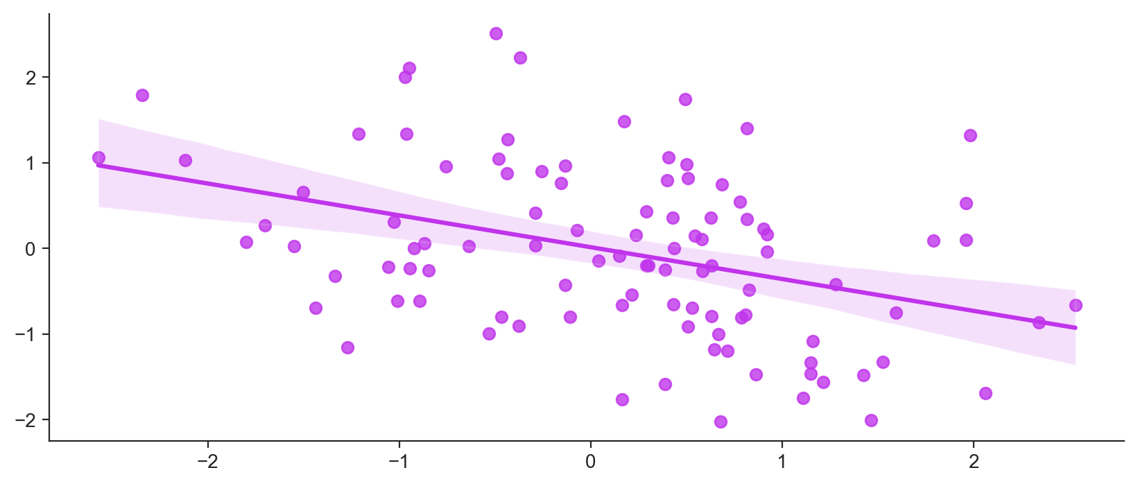
One of the main benefits of linear regression is that it is relatively simple and easy to understand. The coefficients of the independent variables can be used to estimate the impact of each variable on the dependent variable. Linear regression can also handle multiple independent variables, making it useful for modeling complex relationships between variables. Additionally, linear regression is also computationally efficient and can be applied to large data sets with the results of linear regression able to be easily visualized using a scatter plot, which makes it easy to spot patterns and trends in the data. Furthermore, linear regression can be used as a benchmark model to compare with other more complex models.
Below you can see an example from the Scikit-Learn documentation on using Linear Regression:
import numpy as np
from sklearn.linear_model import LinearRegression
X = np.array([[1, 1], [1, 2], [2, 2], [2, 3]])
# y = 1 * x_0 + 2 * x_1 + 3
y = np.dot(X, np.array([1, 2])) + 3
reg = LinearRegression().fit(X, y)
reg.score(X, y)

reg.coef_

reg.intercept_

reg.predict(np.array([[3, 5]]))
Polynomial Regression
Polynomial regression is a form of regression analysis in which the relationship between the independent variable x and the dependent variable y is modeled as an nth degree polynomial. It allows for more flexibility to model non-linear relationships between variables, unlike linear regression which assumes that the relationship is linear. Below you can see the generalized equation for polynomial regression, where y is the dependent variable, and the x values would be the independent variables. Notice how we could expand this by choosing higher orders of polynomials (to some order k) and we could have also included interaction terms.
One of the key advantages of polynomial regression is its ability to model non-linear relationships. This method can capture more complex patterns and trends in the data, leading to more accurate predictions. Moreover, it allows for the modeling of interactions between variables, which can be useful in many applications. It is important to note that polynomial regression has its own set of assumptions and overfitting could occur if the degree of polynomial is too high.
If you choose too high of a polynomial degree you may find yourself overfitting to your training data. You will want to test several different choices for degrees and compare results from both your training set and your test set to fully evaluate your model. It is also good practice to compare the results of polynomial regression with other models such as linear regression to check if you are actually getting a performance boost from using polynomial regression (which is slightly more computationally intensive than linear regression).
Below you can see an example from the Scikit-Learn documentation on using PolynomialFeatures to generate the polynomial version of the feature set, which you could then feed into a Linear Regression:
import numpy as np
from sklearn.preprocessing import PolynomialFeatures
X = np.arange(6).reshape(3, 2)
X


poly = PolynomialFeatures(2)
poly.fit_transform(X)


poly = PolynomialFeatures(interaction_only=True)
poly.fit_transform(X)
Something that is important to note from the above is that you can technically create a polynomial feature set and apply other regression methods to it, such as Ridge, LASSO, or Elastic-Net regression.
Ridge Regression
Ridge Regression is a variation of linear regression that addresses some of the issues of linear regression. Linear regression can be prone to overfitting when the number of independent variables is large, this is because the coefficients of the independent variables can become very large leading to a complex model that fits the noise of the data. Ridge Regression solves this issue by adding a term to the linear regression equation called L2 regularization term, also known as Ridge Penalty, which is the sum of the squares of the coefficients multiplied by a regularization parameter lambda.
The equation for Ridge Regression can be represented as:
By adding this term, Ridge Regression penalizes large coefficients by squaring them, which helps to prevent overfitting and improve the generalization of the model. The regularization parameter lambda controls the strength of the regularization, a high value of lambda will make the coefficients smaller and a low value of lambda will make the coefficients closer to the linear regression coefficients.
Ridge Regression also has the advantage of being computationally efficient and it can handle multicollinearity (when independent variables are highly correlated).
Below you can see an example from the Scikit-Learn documentation on using Ridge Regression:
from sklearn.linear_model import Ridge
import numpy as np
n_samples, n_features = 10, 5
rng = np.random.RandomState(0)
y = rng.randn(n_samples)
X = rng.randn(n_samples, n_features)
clf = Ridge(alpha=1.0)
clf.fit(X, y)
LASSO Regression
Similar to Ridge regression, LASSO (Least Absolute Shrinkage And Selection Operator) is another variation of linear regression that addresses some of the issues of linear regression.
It is used to solve the problem of overfitting when the number of independent variables is large. Lasso Regression adds a term to the linear regression equation called L1 regularization term, also known as Lasso Penalty, which is the sum of the absolute values of the coefficients multiplied by a regularization parameter lambda.
The equation for Lasso Regression can be represented as:
By adding this term, Lasso Regression penalizes large coefficients, but unlike Ridge Regression, it can also make some of the coefficients equal to zero, effectively performing feature selection. This means that Lasso Regression can help to select the most important variables and eliminate the less important ones. The regularization parameter lambda controls the strength of the regularization, a high value of lambda will make more coefficients equal to zero and a low value of lambda will make the coefficients closer to the linear regression coefficients.
Below you can see an example from the Scikit-Learn documentation on using LASSO Regression:
from sklearn import linear_model
clf = linear_model.Lasso(alpha=0.1)
clf.fit([[0,0], [1, 1], [2, 2]], [0, 1, 2])

print(clf.coef_)

print(clf.intercept_)
Keep in mind that lasso regularization is easily extended to other statistical models including generalized linear models, generalized estimating equations, proportional hazards models, and M-estimators.
Elastic Net Regression
Elastic Net Regression is a hybrid of Ridge Regression and Lasso Regression that combines the strengths of both. It addresses the problem of overfitting when the number of independent variables is large by adding both L1 and L2 regularization terms to the linear regression equation.
The equation for Elastic Net Regression can be represented as:
By adding both L1 and L2 regularization terms, Elastic Net Regression can balance the strengths of Ridge Regression and Lasso Regression. It can make some of the coefficients equal to zero, like Lasso Regression, and it can shrink the other coefficients, like Ridge Regression. The regularization parameter lambda controls the strength of the regularization, a high value of lambda will make more coefficients equal to zero and a low value of lambda will make the coefficients closer to the linear regression coefficients.
Below you can see an example from the Scikit-Learn documentation on using Elastic Net Regression:
from sklearn.linear_model import ElasticNet
from sklearn.datasets import make_regression
>>>
X, y = make_regression(n_features=2, random_state=0)
regr = ElasticNet(random_state=0)
regr.fit(X, y)

print(regr.coef_)

print(regr.intercept_)

print(regr.predict([[0, 0]]))
Decision Tree Based Regression
Decision tree based regression is a method that uses decision trees to model the relationship between a dependent variable and one or more independent variables. Decision Trees are widely used machine learning algorithms that can be used for both classification and regression problems in python.
A decision tree is a tree-like structure where each internal node represents a test on an attribute, each branch represents an outcome of the test, and each leaf node represents a predicted value or class.
In decision tree-based regression, the decision tree is built using the independent variables to predict the continuous dependent variable. The tree is built by recursively partitioning the data into smaller subsets, based on the values of the independent variables. The decision tree algorithm tries to find the best split point for each attribute by minimizing a cost function such as the mean squared error. The tree can be grown to any depth, and the final tree will consist of a set of decision rules that can be used to predict the value of the dependent variable.
Decision tree-based regression has several advantages, such as it can handle both categorical and numerical independent variables, it can handle missing data and it is easy to interpret. It’s important to note that decision tree-based regression is one of the tree-based algorithms available for regression, and it’s good practice to compare the results with other tree-based algorithms such as Random Forest and Gradient Boosting.
Below you can see an example from the Scikit-Learn documentation on using Decision Tree based Regression:
from sklearn.datasets import load_diabetes
from sklearn.model_selection import cross_val_score
from sklearn.tree import DecisionTreeRegressor
X, y = load_diabetes(return_X_y=True)
regressor = DecisionTreeRegressor(random_state=0)
cross_val_score(regressor, X, y, cv=10)
Support Vector Regression (SVR)
Support Vector Regression (SVR) is a type of Support Vector Machine (SVM) algorithm, which is a supervised learning algorithm that can be used for regression problems. SVR is a linear model that aims to find the hyperplane that maximally separates the data points into two classes, while at the same time minimizing the classification error. In SVR, the goal is to find the hyperplane that maximally separates the data points from the prediction error, while at the same time minimizing the margin of deviation between the predicted value and the true value of the dependent variable.
The optimization problem of SVR can be formulated as:
Where the constraints are:
One of the main advantages of SVR is its ability to handle non-linear and non-separable data by using kernel trick. SVR applies a kernel function to the data, which maps the original data into a higher-dimensional space where it can be separated by a linear boundary. This allows SVR to model complex relationships between variables and make accurate predictions.
Another advantage of SVR is its robustness to outliers. SVR uses a cost function that penalizes large errors, which makes it less sensitive to outliers than traditional linear regression methods.
In order to test our Support Vector Regression, you don’t need to be an expert in the above, you can simply test it out with Scikit-Learn! Below you can see an example from the Scikit-Learn documentation on using Support Vector Regression (also notice the scaling used in this example):
from sklearn.svm import SVR
from sklearn.pipeline import make_pipeline
from sklearn.preprocessing import StandardScaler
import numpy as np
n_samples, n_features = 10, 5
rng = np.random.RandomState(0)
y = rng.randn(n_samples)
X = rng.randn(n_samples, n_features)
regr = make_pipeline(StandardScaler(), SVR(C=1.0, epsilon=0.2))
regr.fit(X, y)
If you’re interested in learning more about a vareity of regression and machine learning methods, check out our machine learning course offerings! Such as Python for Machine Learning: